By Keith Millis, Case Caulfield, and Andrea Crook, P.Geoph.
Restrictions to seismic acquisition increasingly limit the positioning of both sources and receivers at theoretically prescribed locations. Designing and subsequently repositioning station locations with respect to those restrictions has become an important and time-conscience aspect of both land and marine seismic programs. Historically, deviations from theoretical locations are prescribed in a set of station positioning guidelines, such as skid and offset guidelines or bingo-card methods (Cooper, 2004). These methods are surface-based approaches and relate to theoretical locations. They make assumptions that may not provide an optimal station location. A new sub-surface based method for optimizing station locations that utilizes sampling and imaging criteria is presented, with benefits of its use highlighted in a case study.
Introduction
Seismic acquisition parameters are typically established by a thorough review of existing seismic data, as well as the use of theory and/or modeling to determine the expected waveform. This analysis leads to a set of imaging requirements – trace density, distribution and statistical diversity – for a given program. A full wavefield design consists of sources and receivers positioned so as to generate midpoints with a full complement of offsets and azimuths. Figure 1 shows the theoretical layout, and resulting offset-azimuth distribution for a particular bin. The rays in the spider plot, and corresponding dots in the polar azimuth plot, correspond to the offset (distance from center) and bearing (towards the receiver) for all of the traces within the bin.
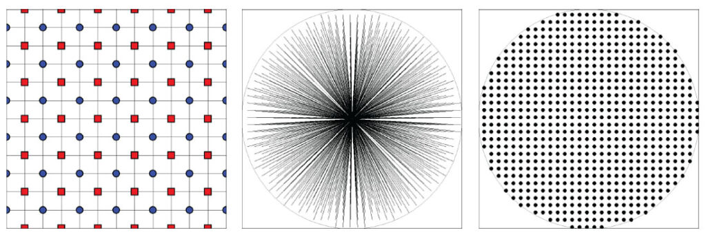
Figure 1. The left panel shows a full wavefiled layout of sources in red and receivers in blue, overlaying the corresponding natural bin grid. The middle panel has zoomed in to a specific bin and drawn the spider plot, in which a ray is drawn for each source-receiver pair from the center toward the receiver – representing azimuth – and whose length corresponds to the offset. The right panel is similar to the spider plot with dots drawn at the ends of the rays of the spider plot. Their polar location corresponding to the bearing toward the receiver, and distance from the center corresponding to the offset.
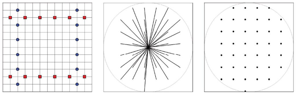
Figure 2. The left panel shows the full wavefield design decimated into lines and stations, with the receivers in blue, and sources in red overlaying the natural bin grid. The middle and right panels shows the decimated offset and azimuth content of the same bin in Figure 1.
Skid and Offset Guideline Issues
In a CMP scatter, or bin fractionation design (Cordsen, 2000), the distance in which a station can move from its theoretical location while contributing to the same bin is dependent on the direction of the movement. With a double scatter design, which has four theoretical midpoints in each bin, in order to keep the midpoints in their original bins the stations can only move one half of a bin dimension in one direction, but three halves of the bin dimension in the opposite direction, shown in Figure 3. Skid and offset guidelines do not capture these complexities, and depending on the choice of bin grid orientation, the station movements will result in CMPs drifting out of the intended bin and fold imprints will be in the final dataset.
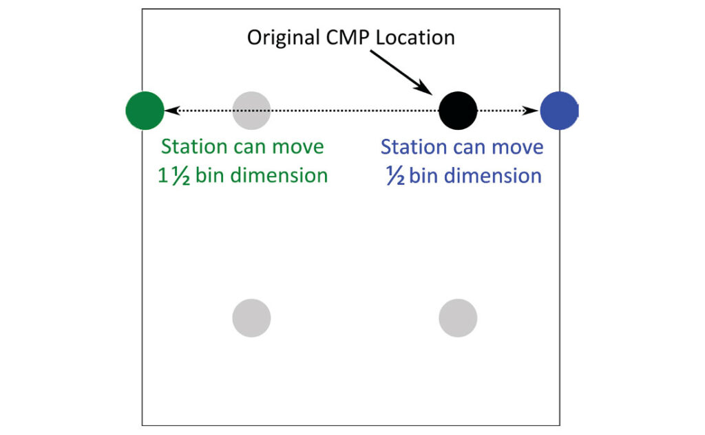
Figure 3. A double stagger layout is designed to have four theoretical CMP locations within a bin. Depending on the CMP, the contributing stations are limited in where they can be located and any movements of those stations becomes directionally dependent.
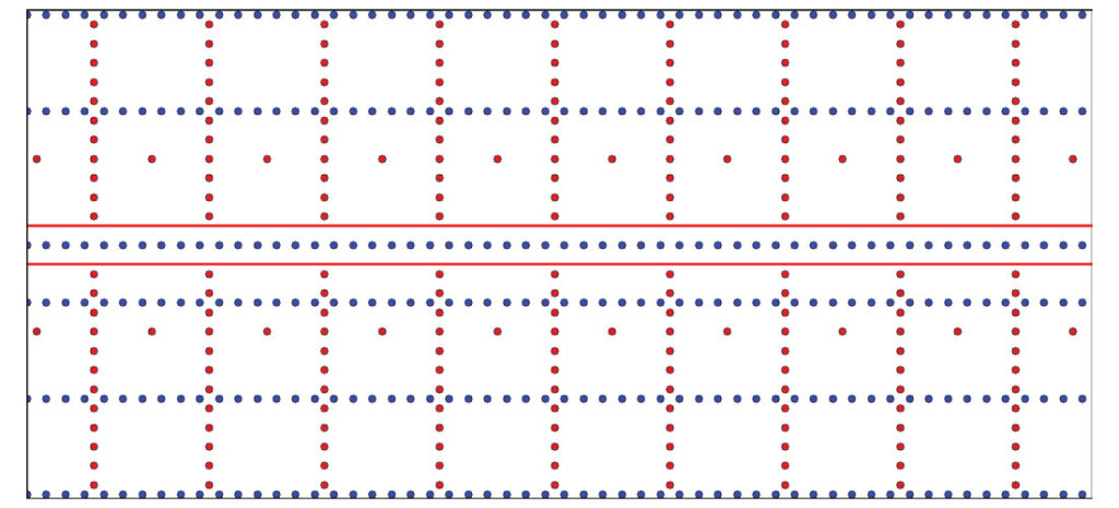
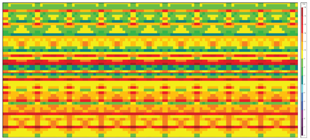
Figure 4. The top panel shows a source restriction outlined with red lines, and its effect on the layout of sources (red) and receivers (blue). The receiver line has been offset from theoretical. This example occurs frequently in seismic acquisition where vegetation for a pipeline right-of-way has been cleared. The resulting fold plot is shown in the bottom panel. Note the significant fold stripe that results from improperly positioned sources.
ORM Method
Consider a distribution of midpoints that has been chosen as a manner of adequately sampling the seismic waveform. By convention they are binned according to established imaging criteria, which yields a comprehensive set of bin attributes, such as trace locations within the bin, trace density, offset and azimuth. The populated bin grid completely describes the layout geometry of sources and receivers.
By limiting where stations can be positioned, surface restrictions, by proxy, limit the trace density, trace location and associated offset and azimuth distribution within the bin. Restrictions can be projected into bin space and viewed in a polar azimuth diagram. Doing so indicates what trace diversity is available to a particular bin under a given framework of restrictions. A circular restriction that affects the theoretical layout of stations is shown in figure 5. If the restriction affects only sources, only receivers, or both, the traces enclosed by the red, blue, or both circles respectively, cannot be recovered. It should be determined if the content of the traces affected by the restriction can be dropped, or if alternate station locations are warranted. Assuming that the identified restriction is the only limitation to positioning sources and receivers, the affected traces can be translated toward the origin, which affects offset; rotated about the origin, which affects azimuth; or a combination of both. In fact, many potential offset-azimuth combinations can be established and ranked in order of the expected impact on the resulting seismic image.
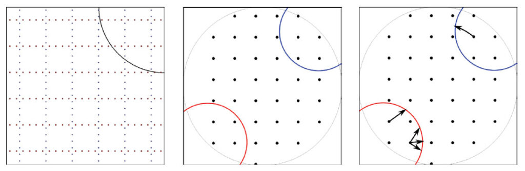
Figure 5. The left panel shows a layout of sources (red) and receivers (blue), with a circular restriction in the North-East (upper-right) corner. The middle panel shows the theoretical offset and azimuth distribution for a given bin. The circular restriction has been projected into “bin-space” and coloured red or blue indicating which offset-azimuth combinations are affected if the restriction affects sources or receivers respectively. The right panel shows how repositioning source-receiver pairs can affect only offset (left-most trace), azimuth (right-most trace) or a combination of both (bottom-most trace).
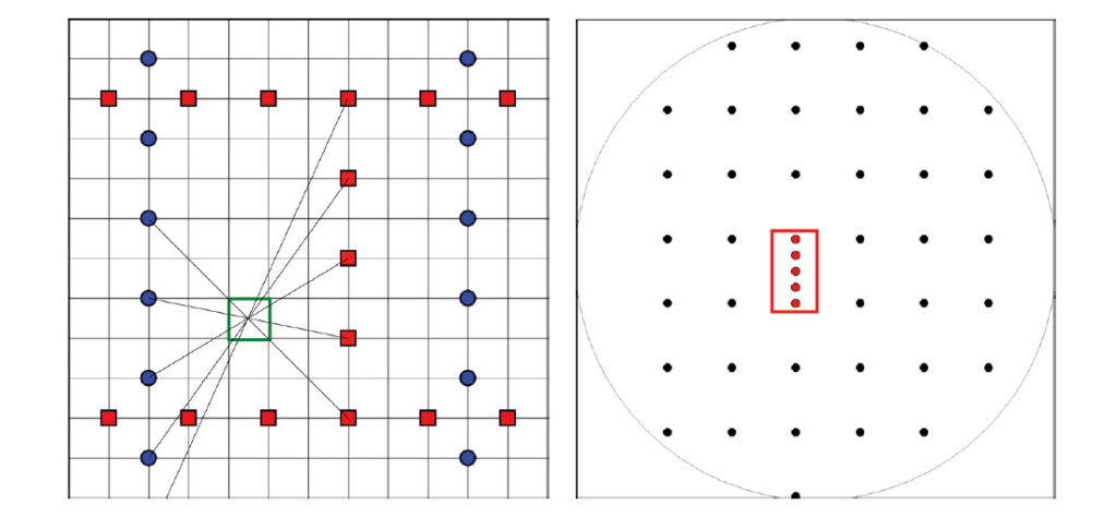
Figure 6. Repositioning a source, as seen in the left panel, can be constrained to only those positions where a reciprocal receiver exists to complete the pair. That is, a trace can be added to a bin without having to reposition or add both a source, and a receiver. Assuming the receivers are at theoretical locations, the resulting offset and azimuth contributions are shown in the right panel.
For a given survey there can be several restrictions affecting many bins. In some cases, there may be hundreds of possible source-receiver pairs that satisfy the specified imaging requirements for a given bin. Some of these results may also contribute positively to the trace content in other bins. To objectively choose one set of station locations over another requires a sophisticated ranking scheme for the output. With so many potential station locations, the process of ranking and selecting optimal station locations can only be done algorithmically. If a potential source-receiver pair improves the trace density or statistical diversity within a bin, and also contributes a desired set of offsets or azimuths in a neighboring bin, its effective rank increases. Assessing a group of bins whose trace contents are sub-optimal, determining whether source-receiver pairs exist that can improve the content within each bin, and ranking the resulting locations by effectiveness of contributing traces in the group of bins as a whole leads to the resulting optimal restriction model. The ranked stations can be automatically selected on a contribution basis or on the basis of operational feasibility, and subsequently implemented into the acquisition.
Case Study
The ORM method was used on a recently acquired 3D, which was shot to identify horizontal drilling targets and subtle bypassed pay areas in a relatively shallow Mississippian carbonate field. Target depths were approximately 700-800m. The data is very high frequency with upper limits of 180 Hz and was processed at 1 msec. The pay zones require careful structural understanding to guide horizontal wells; optimization can depend on subtle amplitude changes that indicate facies and porosity changes. In addition, wavelet analysis and inversion have been used to understand production trends.
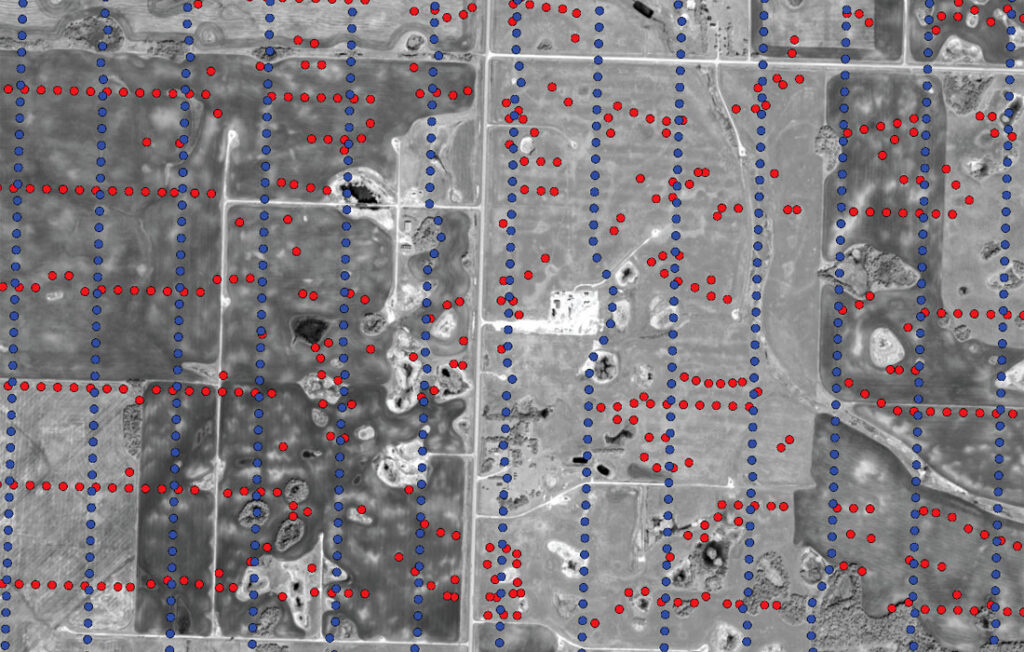
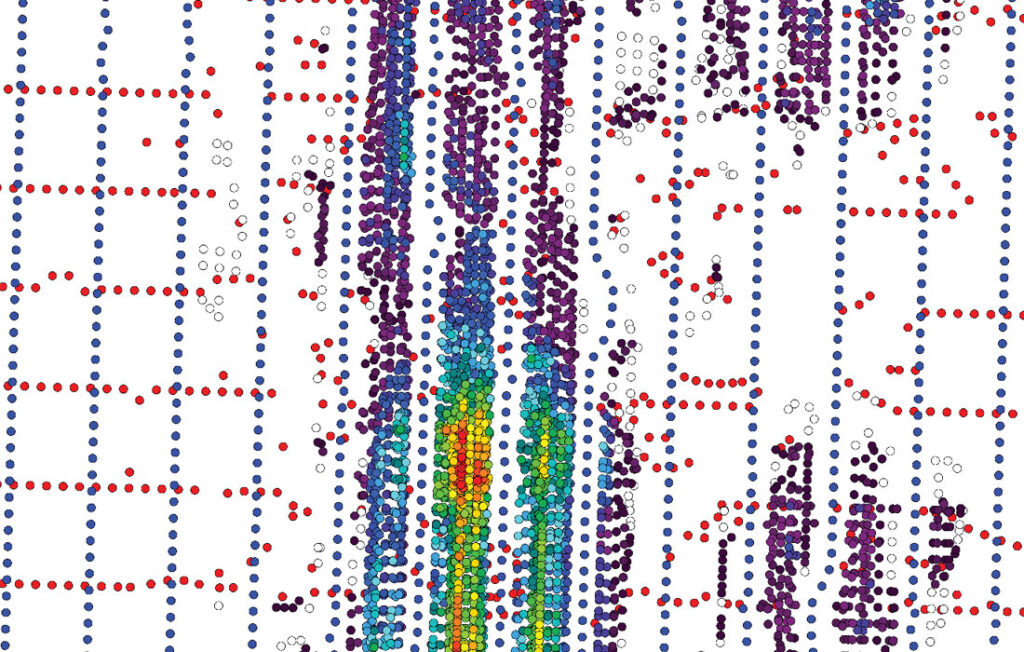

Figure 7. The top panel shows the layout of sources (red) and receivers (blue) as they had been surveyed. The middle panel shows all of the possible locations where receiver infill stations can benefit the acquisition, coloured according to their effectiveness at fulfilling the specified imaging criteria. Receiver station locations were automatically selected from the possibilities, shown in the bottom panel as green circles.
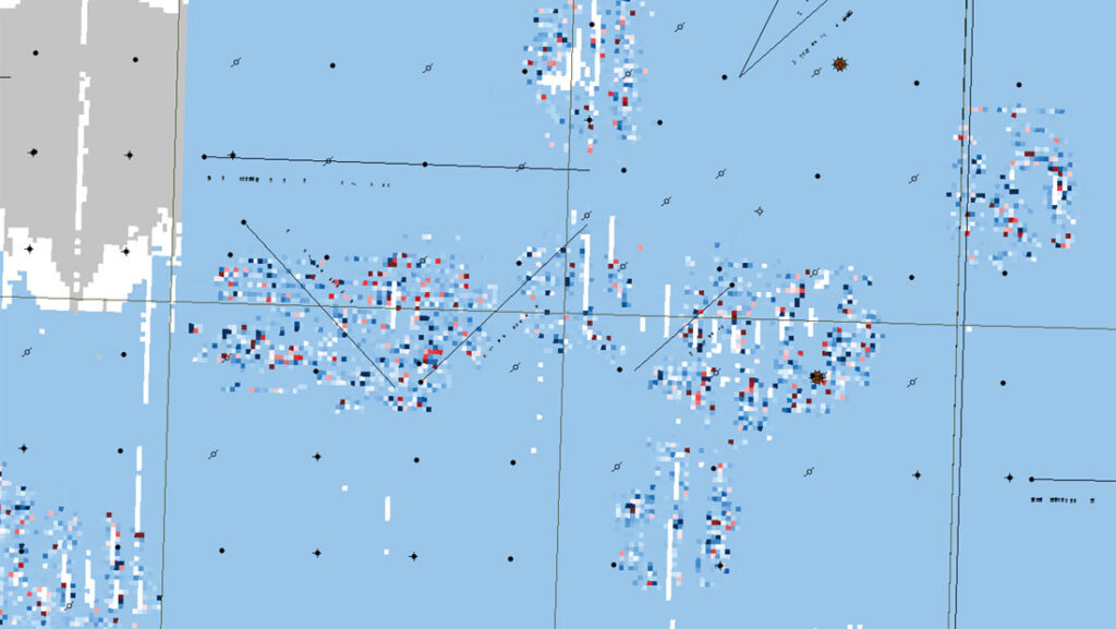
Figure 8. This image shows the ratio of amplitudes of unmigrated time slices near the target level between the data with and without the infill receivers at ORM optimized locations. Clearly showing the prominence of amplitude effects in the data when infill stations are not present, this source of error could have significant exploration consequences.
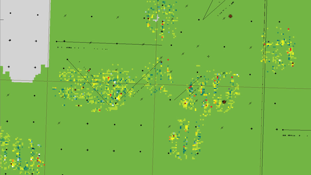
Figure 9. This image shows the time difference between the same horizon using the data with and without infill receivers.
Conclusion
To properly account for surface complexities in seismic acquisition, reshaping the surface design process from a station movement framework that is based on “area of responsibility” and does not account for the location of other stations within the survey, to a method that is driven by attribute and imaging objectives has been presented. The ORM method provides station locations that have been optimized algorithmically, and are based on imaging requirements. Improving upon the resulting seismic image, the ORM method has shown to increase confidence in both time structures and amplitudes. Additionally, improving the efficiency of station placement leads to more streamlined operational processes.
The authors would like to thank Corex Resources Ltd., and Crescent Point Energy for permission to use their data. We would also like to thank Sara Dobek and Regan Kennedy at Earth Signal Processing, and Cameron Crook at OptiSeis™ Solutions Ltd. for their contributions.