By Keith Millis, Cameron Crook
Summary
Surface restrictions to seismic acquisition increasingly limit the ability to place stations at their theoretical locations. Consequently, the acquisition design process is faced with increased pressure to model programs with surface perturbations in mind (Cooper, 2004). An optimal restriction modeling method requires reshaping the surface design process to one that is driven by sampling, attribute and imaging objectives, and also respects restrictions and operational efficiencies. Introduction As a seismic image can be greatly affected by surface restrictions, a significant amount of effort should be placed on determining the optimal location of each seismic station. Due to the time sensitive nature of seismic operations and changing field conditions this process is often handled in the field by following a set of positioning guidelines. Station positioning guidelines, commonly referred to as “Skid and Offset Guidelines” attempt to account for potential restriction scenarios during the acquisition of the program. If a large, complex or overlapping set of restrictions is encountered, communication between the field crew and acquisition geophysicist may occur. There are several pitfalls in this approach relative to imaging objectives that include misplaced stations due to common midpoint stagger, station movements that do not consider surrounding station locations, and redundant station placement. To improve operational efficiency and eliminate the issues mentioned above, a new method is presented.
Method
Sampling requirements determined in the parameter selection stage of the design process are attributes that drive the Optimal Restriction Model (ORM) algorithm and resulting station locations. The method can be performed as a two-step process with optimal station locations produced both before, and concurrent with, work in the field. The first iteration can be successful in determining feasibility of seismic acquisition in heavily restricted environments. The second, and any subsequent iteration, will produce final station locations based on surveyed restriction information, subject to the imaging and operational constraints driving the acquisition.
After development and optimization of theoretical parameters, the program is mapped at real-world coordinates. Set-back distances from houses, concrete structures, waterways, power lines, pipelines, as well as pertinent environmental mandates, stakeholder considerations, slope contours and other restrictions can be ascertained with their locations and extent also mapped.
With a focus on spatial continuity, theoretical stations affected by the restrictions can be offset perpendicular to the line bearing. Particular attention should be given to the continuity of stations and resulting “smoothness” of the line that results from the station movements (Vermeer, 1997). Figure 1 shows the process of defining a Gaussian function with a defined value for the “full width at half maximum”, for every station along a given line. Taking the maximum value of all relevant functions at each station location produces a sufficiently smooth result to project the stations onto. Any stations that cannot be offset within defined parameters will be addressed later in this method and temporarily excluded.
Examples
Common Midpoint (CMP) scatter or bin fractionation designs position the stations so as to achieve an organized CMP distribution within the bins (Cordsen, 2000; Cooper, 2004). In such a design, the distance in which a station can move from its theoretical location while contributing to the same bin is dependent on the direction of the movement. Figure 2 shows a double stagger CMP distribution within a bin. If a surface restriction impedes the placement of a station at its theoretical location, in order to keep the midpoints in their original bins the station can move one half of a bin dimension in one direction, but three halves of the bin dimension in the opposite direction. Skid and offset guidelines do not always capture these complexities, and depending on the choice of bin grid orientation, the station movements will result in CMPs drifting out of the intended bin and fold imprints in the final dataset. By solving for attribute gaps within each particular bin, recommended station locations will be constrained to ones that generate CMPs within that bin, or fractionated locations within the bin.
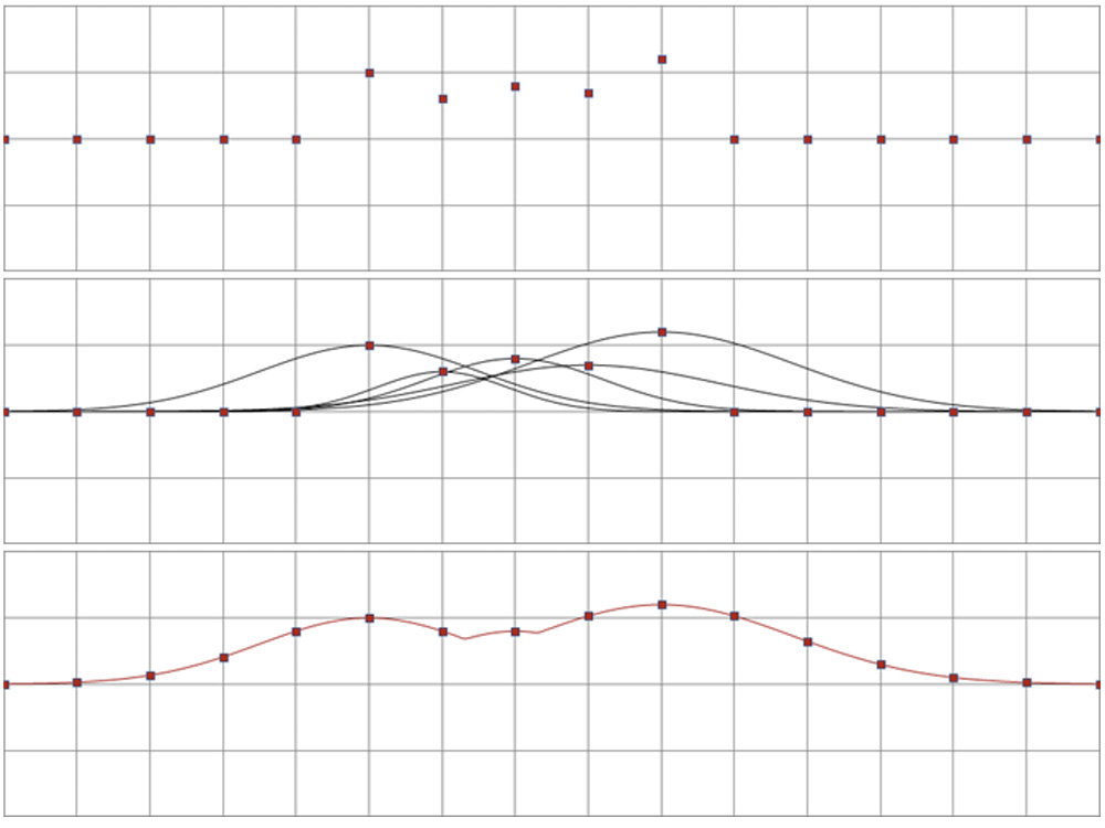
Figure 1: Top Frame – A set of sources that have been offset from theoretical. Middle Frame – a Gaussian function is defined at every source station location along the source line. Bottom Frame – each source station is projected onto the maximum result of each Gaussian function resulting in a “smooth” line.
CMP information resulting from the new station locations are then binned and queried to determine the trace count, and statistical diversity the bins contain. Depending on the coverage and sampling requirements, optimal locations for the excluded stations, or any additional stations, are determined by filling the gaps apparent in the bin query and testing the restriction validity of the recommended locations.
Since there may be a large set of unique and non-unique station locations that result from the bin query step, a sophisticated system of ranking potential locations is required. Ranking systems may be general and include unique offset and azimuth criteria, or defined by imaging or processing objectives. These objectives may include sampling with respect to interpolation inputs, pre-stack attributes, or a populated bin grid with trace offsets and azimuths matching a previous acquisition (4D repeatability). After these results have been ranked, they are can be automatically selected from within the ranked arrays.
Figure 2: Top-right panel – Double stagger layout, sources are coloured red, receivers blue. Top-left panel – blown up view of a bin grid showing organized CMP scatter. Bottom-right – movement of one particular source North ½ a bin grid dimension, and also South by 1 ½ a bin grid dimension. Bottom-left – CMP location from source movements are now located at the bin edge.
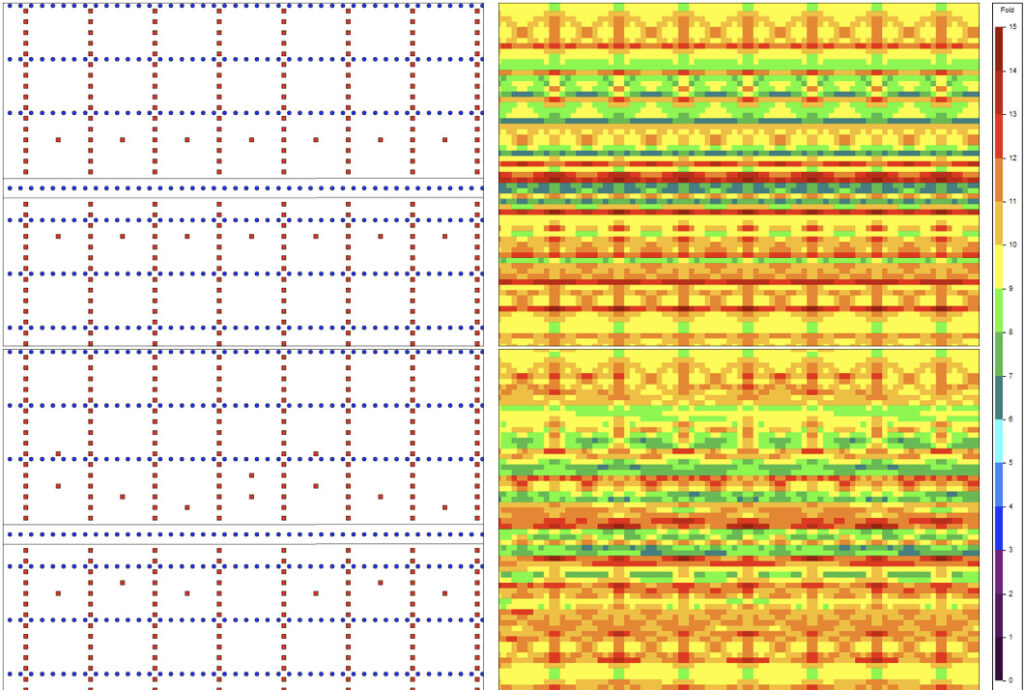
Figure 3: Top-left panel – an East-West receiver line has been offset off of its theoretical location, and sources have followed typical skid and offset guidelines. Top-right panel, the resulting fold from the movements in the top-left panel. Bottom-left panel – the receiver line has moved, but sources have now been positioned using the optimal restriction modeling method. Bottom-right panel – the fold that results from the movements in the bottom-left panel.
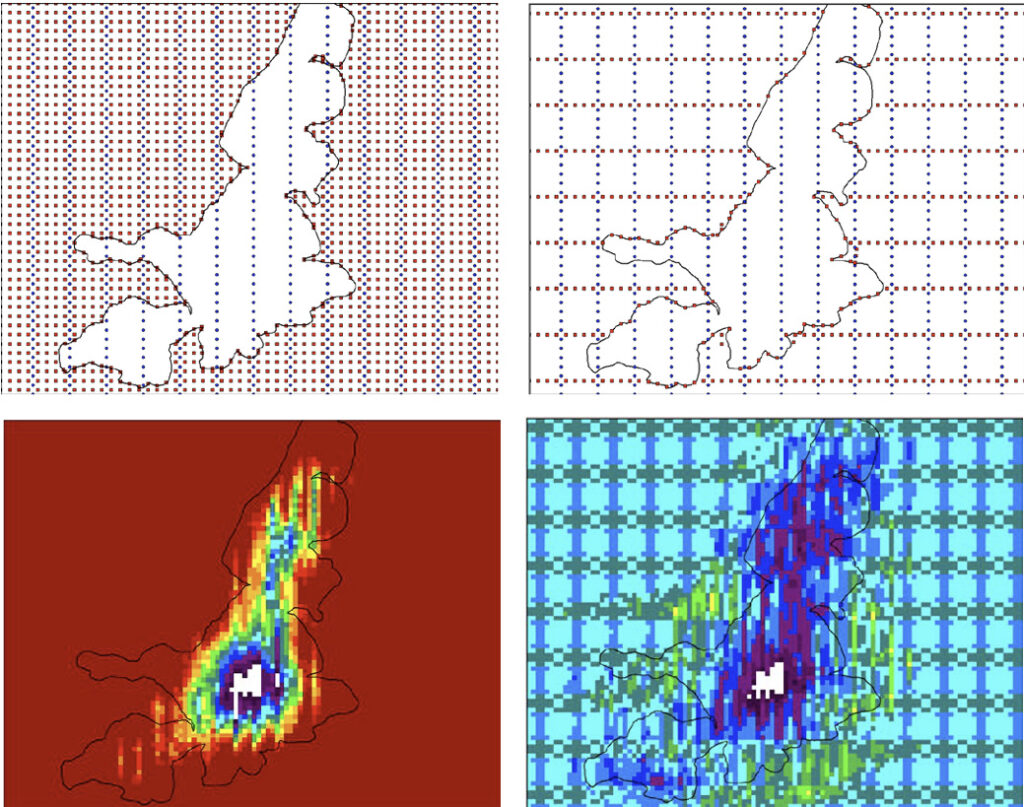
Figure 4: Top-Left Panel – Every available “full wavefield” location for a source outside of a restriction is being used. Top-Right Panel – optimal restriction model layout for a given set of attribute constraints. Bottom-Left Panel – fold plot from top panel layout. Bottom-Right Panel – fold plot from optimal restriction model layout. Note that zero fold bins are now filled and a more even trace distribution across the restriction.
Conclusion
To properly account for surface complexities in seismic acquisition, reshaping the surface design process from a station movement framework that is without respect to bins or the location of other stations within the survey, to a method that is driven by attribute and imaging objectives has been presented. The ORM method provides station locations that are optimized algorithmically, avoids redundant locations, and meets imaging requirements. Improving the efficiency of station placement leads to improved operational processes. The method can also be used for improving sampling of time-lapse programs as new infrastructure relative to the legacy survey is constructed.